CS224N NLP with Deep Learning
讲课的老师是大名鼎鼎的 Christopher Manning,NLP 领域的开拓者之一。我很喜欢他的澳洲口音,不像英式口音的生疏内敛,也不像美式口音的横冲直撞。听他讲课有一种在乡下听老爷子谈天说地之感。
This article is a self-administered course note.
It will NOT cover any exam or assignment related content.
Word Embeddings
将 tokens 从 human-interpretable (words) 转为 machine-interpretable (word vectors/embeddings)。
Discrete symbols. e.g., 使用 one-hot encoding。缺点很明显:vector 稀疏且维数高;丧失了词之间的相似性信息。
Distributional semantics. A word's meaning is given by the words that frequently appear close-by. 模型大致分为两种:Direct prediction model 与 Count-based model。
Evaluation of word embeddings.
- Intrinsic Evaluation. e.g., Analogy Evaluations, Correlation Evaluation.
- Extrinsic Evaluation. e.g., Sentiment Analysis, Named-entity Recognition (命名实体识别). 概念有点像下游任务。当 extrinsic task 提供的数据足够大时,可以对训练出的 word embeddings 进行 fine tune。
Direct Prediction: Word2Vec
滑动窗口逐个扫过 corpus。窗口的中心词 (center word) \(w_c\),上下文词 (outside word) \(w_o\)。
对于所有词 \(w_x\in \text{Vocab}\),其 word vector 有两种表示 \(u_x \in U, v_x\in V\)。\(U\to R^{n\times d}\) 是周围词向量,\(V\to R^{n\times d}\) 是中心词向量。我们把 \(U\) 和 \(V\) 统称为 \(\theta\),它们既是需要学习的参数,也是最终得到的结果 (词向量为 \(U,V\) 取平均)。
基于 naive softmax 定义的目标函数 (objective function) - 该函数由词间的相似度 (likelihood) 取 log 整理而成。 \[ J(\theta)=-\frac{1}{T}\sum_{t=1}^{T}\sum_{-m\leq j\leq m,j\neq 0} \log P(w_{t+j}|w_{t};\theta) \] 给出中心词 \(c\),上下文词为 \(o\) 的概率分布 \(P(o|c)\) 定义如下 (就是 softmax): \[ P(o|c)=\frac{\exp(u_o^Tv_c)}{\sum_{w\in \text{Vocab}} \exp(u_w^T v_c)} \] 计算梯度 (以参数 \(v_c\) 为例,过程见 pp.39) 可以发现它本质上是 观测值 (observed) - 期望值 (expected): \[ \frac{\partial}{\partial v_c} \log(P(o|c))=u_o-\sum_{x=1}^v P(x|c) u_x \] 有 corpus,有目标函数 \(J(\theta)\),梯度下降更新 \(\theta\) 即可。但在 naive softmax 定义下,每次更新都要计算所有 \(\theta\) 的梯度,还要计算成本很高的 \(\sum_{w\in \text{Vocab}} \exp(u_w^T v_c)\),计算负担很大。为解决这个问题:
- 使用 Stochastic Gradient Descent 进行梯度下降,每次窗口滑动都更新 \(\theta\)。
- 使用 Negative Sampling。修改目标函数 \(J(\theta)\),将枚举到的 co-occurring 中心词-上下文词对 \((c,o)\) 作为正样本,再随机选取 \(k\) 个负样本 \((c, o_{neg})\),最大化 \(P(o|c)\) 的同时最小化 \(P(o_{neg}|c)\)。
- Stochastic gradients with negative sampling。使用 SGD + 负采样的 Word2Vec 算法,半径为 \(m\) 的窗口每滑动一次,仅更新 \(2m+1\) (window words) 加上 \(2mk\) (negative words) 个参数即可。
Word2Vec 的两种范式。
- Skip-grams (SM) model:给出中心词 \(c\),预测上下文词 \(o\) 的概率分布。
- Continuous Bag of Words (CBOW):给出上下文词 \(o\),预测中心词 \(c\) 的概率分布。Bag of words 意味着模型对每个位置的预测都相同。
Count-based: Co-occurrence Matrix
一个更直接,更自然的想法:既然 center word 的含义与 outside words 有关,为何不直接使用 outside words 的词频作为 word embeddings?
我们直接统计 (两种方式) 出共现矩阵 (co-occurrence matrix) \(X\),\(X_{ij}\) 表示以 \(w_i\) 为 center,\(w_j\) 为 outside word 的频率。直接取 \(X_i\) 作为 \(w_i\) 的 word embedding。
这样做的问题很明显,也涌现了对应的修正方案:
- \(X_i\) 维数太高,和词汇表大小等同 \(\to\) 对 \(X\) 进行 Singular Value Decomposition (SVD) 实现 Dimensionality Reduction。
- function words 如 the, he, has 出现频率太高,不利于对语义而非语法的捕捉 \(\to\) 对频率取 log,设置最低频率,或干脆忽略 function words。
- 统计词频时,给予离中心词较近的词更高的权值。或使用 Pearson correlation 而非纯计数进行统计 (这样做的话记得把负值置 0)。
COALS 模型就采用了 count-based 架构,效果超过了部分 Word2Vec 模型。
GloVe
比较 Direct Prediction 与 Count-based 架构的优劣:
- window-based 的直接预测架构 (e.g., skip-gram, CBOW) 在捕捉复杂的语义模式和词性相似度上表现优秀,但无法利用 global co-occurrence statistic。
- count-based 的矩阵分解架构 (e.g., LSA, COALS) 能够有效利用 global statistical information,却在 word analogy 等任务上表现差。这说明其 vector space 结构的 sub-optimal。
GloVe (Global Vectors for Word Representation) 则集两家之长:Using global statistics to predict the probability of word \(j\) appearing in the context of word \(i\) with a least squares objective.
GloVe 架构中既有 \(U,V\) 两个 word embedding 空间,又有共现矩阵 \(X\)。其目标函数为: \[ J(\theta)=\sum_{i=1}^{W}\sum_{j=1}^W f(X_{ij})(u_j^Tv_i-\log X_{ij})^2 \] 具体的推导过程见 notes2 - word2vec。还是比较 convincing 的。
Neural Networks
NN (这里主要讲的是 MLP) 的概念已经非常熟悉了,不赘述。
Feed-forward Computation (正向计算).
Backpropagation (反向传播).
- Use Jacobian form (Jacobian Matrix 雅可比矩阵,可以视作是矩阵意义下的导数) as much as possible, reshape to follow the shape convention (参数和其梯度的形状一致) at the end.
- 一个公式总结反向传播:downstream gradient = local gradient * upstream gradient.
Manual Gradient Checking: Numeric Gradient. 使用数值微分的方式验证自动微分的正确性。
训练 NN 时的 tricks.
- Regularization aka Weight Decay. 加入正则项阻止模型过拟合。
- Dropout. 以 \(p\) 的概率丢弃某个 neuron,\(1-p\) 的概率使某个 neuron 的输出除以 \(1-p\)。这是为了使得应用 dropout 前后丢弃层的输出期望一致。此外,在做 inference 时不启用丢弃层。
- 其他激活函数中的 Leaky ReLU。\(\text{leaky}(z)=\max(z, k\cdot z) \ \ (0<k<1)\):这样当 \(z\leq 0\) 时也允许有 small error 反向传播回去。
数据预处理的 tricks. Mean Subtraction, Normalization and Whitening.
Parameter Initialization.
- Normal distribution around 0
- Xavier Initialization. 维持层间 activation variances 与 backpropagated gradient variances 的稳定性。第 \(l\) 层的权值 \(W\in R^{n(l-1)\times n(l)}\) 使用以下的分布进行随机初始化。
\[ W\sim U[-\sqrt{\frac{6}{n^{(l-1)}+n^{(l)}}}, \sqrt{\frac{6}{n^{(l-1)}+n^{(l)}}}] \]
Learning Strategies (对 optimizer 的研究).
Annealing (退火). 学习率 \(\alpha\) 随着迭代次数 \(t\) 的增加而降低。若初始学习率为 \(\alpha_0\),常见方式有:
- \(\alpha(t)=\frac{\alpha_0 \tau}{\max(t, \tau)}\), \(\tau\) 为超参数。
- 指数衰减 \(\alpha(t)=\alpha_0 e^{-kt}\), \(k\) 为超参数。
Momentum Update. 一个小球的运动方向受当前受力方向 (当前梯度 \(\frac{\partial J}{\partial x}\)) 与原运动方向 (之前的所有梯度累积而成的动量 \(v\)) 共同影响。学习率为 \(\alpha\),动量衰减率为 \(\mu\) (梯度对动量的影响随时间的衰减率,\(t\) 个迭代之前的梯度对当前动量的影响为 \(\mu^t\)),\(\mu\) 常取 0.9, 0.5 等值。 \[ \begin{aligned} v&:=\mu v-\alpha \frac{\partial J(\theta)}{\partial x} \\ x&:=x+v \end{aligned} \] Adaptive Optimization Methods. Each parameter has its own learning rate. Parameters that have not been updated much in the past are likelier to have higher learning rates. 以 AdaGrad 为例,某参数 \(\theta_i\) 在第 \(t\) 次迭代的 (真) 学习率被前 \(t-1\) 次的梯度历史影响。 \[ \theta_{t,i}=\theta_{t-1,i}-\frac{\alpha}{\sqrt{\sum_{\tau=1}^{t}g_{\tau,i}^2}} g_{t,i} \text{ where } g_{t,i}=\frac{\partial}{\partial \theta_{t,i}} J_t(\theta) \] 注意到 AdaGrad 中 (真) 学习率是单调下降的。RMSProp 作为 AdaGrad 的一个变种,利用了 moving average of squared gradients 解决了这个问题。Adam 又是 RMSProp 的一个变种,它使用 momentum-like updates。
Dependency Parsing
非常 linguistic 的内容。下学期想 enroll general linguistic 那门课了。
与机器语言不同,自然语言非常之 ambiguous。避免歧义的前提是了解句子的结构 (典中典之 Students Get First Hand Job Experience),因此句法分析 (syntactic structure analysis) 成为了传统 NLP 领域中的一个重要任务。
语法结构的两种模型:
- Constituency Structure (成分结构).
- Dependency Structure (依赖结构).
Constituency Structure. 基于句子中各词的词性和短语结构语法把单词组织成嵌套的结构 (nested structure),把较小的语言成分按照规则组装为较大的语言成分,表达的意义也随之越来越复杂。
Dependency Structure. 强调词与词之间的依赖关系。依赖关系是一条单向边 \((w_i,w_j,v)\),表示 \(w_j\) 依赖于 \(w_i\),依赖方式是 \(v\) (\(\mathtt{prep,pobj,nsubjpass}\), etc.)。\(w_i\) 被称为 head (governor),\(w_j\) 被称为 dependent (modifier)。分析依赖关系连边后往往会形成一颗依赖树 (dependency tree)。
Dependency Parsing 问题基本来说就是训练一个能够对给定句子生成对应依赖树的模型。
- Learning: Given a training set \(D\) (e.g., Stanford Universal Dependencies) of sentences annotated with dependency graphs, induce a parsing model \(M\) that can be used to parse new sentences.
- Parsing: Given a parsing model \(M\) and a sentence \(S\), derive the optimal dependency graph \(D\) for \(S\) according to \(M\).
Traditional Methods
Dependency Parsing 的传统方法。
- DP, 复杂度 \(O(n^3)\)。
- 基于最小生成树的 parser MSTParser。生成 \(n^2\) 条带依赖概率的边,再使用 MST 进行选择。
- MaltParser: 采取 transition-based parsing 或 greedy deterministic dependency parsing。
Greedy Deterministic Transition-Based Parsing. 该框架下 parser 是一个自动机,贪心的进行状态转移。
先定义状态 (state):对于句子 \(S=w_1...w_n\),状态 \(c=(\sigma,\beta,A)\),\(\sigma\) 是一个栈,\(\beta\) 是一个 buffer,\(A\) 存储所有依赖关系。初始状态 \(c_0\) 为 \(([w_0]_{\sigma},[w_1,...,w_n]_{\beta},\emptyset)\),\(w_0\) 是为方便创造的依赖树根 ROOT。终止状态为 \((\sigma,[]_{\beta},A)\)。
转移 (transitions) 共有三种:
- \(\mathtt{SHIFT}\). 将 buffer 中的第第一个词压入栈中。
- \(\mathtt{LEFT\_ARC}_r\). 若从栈顶开始的两个词为 \(w_j,w_i\),连一条边 \((w_j,r,w_i)\) 并存入 \(A\) 中,从栈中弹出 \(w_i\)。
- \(\mathtt{RIGHT\_ARC}_r\). ...连一条边 \((w_i,r,w_j)\) 存入 \(A\) 中,从栈中弹出 \(w_j\)。
设计好了自动机的状态与转移,接下来应该有一个 deterministic 的决策器指导对于某种状态应该采取什么转移。
Neural Dependency Parser
接下来就是 Manning 和他的学生 Chen Danqi 的工作了:他们设计了一个神经网络作为决策器。这个神经网络以从当前状态 \(c=(\sigma,\beta,A)\) 中抽取的特征作为输入进行一个三分类,根据输出决定下一次转移是 SHIFT,LEFT ARC,RIGHT ARC 中的哪一种。实验结果证明这种 parser 的准确性和效率都大大提高了。
一般来说,我们从当前自动机的状态 \(c\) 中抽取三种特征:\(S_{word}\) 即栈或 buffer 中的某些词,\(S_{tag}\) 即这些词对应的词性 (POS, Part of Speech),\(S_{label}\) 即这些词的 dependents 和对应的依赖关系。
把这三种特征表示成向量 \(x^w,x^t,x^l\) 并 concatenate 成一个低维稠密的分布式向量 \([x^w,x^t,x^l]\) 喂到 NN 中,经过一个隐藏层 (激活函数是 cubic function) 和 softmax 层后得到结果。
题外话,看到 Chen Danqi 这个名字我隐约觉得有点熟悉,查了下才知道她是隔壁雅礼的真 · IOI 巨佬,在高中就发明了 CDQ 分治和插头 DP 这些折磨后世的算法,现在是 Princeton 的 NLP group co-leader......真跪了。
Language Models
终于到了语言模型及其实现。之前在 dive into DL 中囫囵吞枣学到的知识可以好好反刍一下了。
Language Models. 语言模型是一种词语概率分布模型,它能够预测长为 \(m\) 的序列 \((w_1,w_2,...,w_m)\) 的出现概率。应用 \(n\) 阶马尔可夫假设,该概率可表示为: \[ P(w_1,...,w_m)=\prod_{i=1}^m P(w_i|w_1,...,w_{i-1})\approx \prod_{i=1}^m P(w_i|w_{i-n},...,w_{i-1}) \]
Traditional Implementations
\(n\)-gram Language Models. 在拥有足够 corpus 的情况下,\(n\) 元语法语言模型直接使用频率估计概率。以下两个式子分别是 uni-gram 与 bi-gram 语言模型的公式。 \[ P(w_2|w_1)=\frac{\text{count}(w_1,w_2)}{\text{count}(w_1)}, p(w_3|w_1,w_2)=\frac{\text{count}(w_1,w_2,w_3)}{\text{count}(w_1,w_2)} \] \(n\) 元语法模型的缺点:Sparsity and Storage.
- Sparsity problems. 第一种情况 - 分子 \(\text{count}(w_1,w_2,w_3)=0\);改善方法是 smoothing:令分子等于一个小量 \(\delta\)。第二种情况 - 分母 \(\text{count}(w_1,w_2)=0\);改善方法是 backoff:减小 \(n\),转而使 \(\text{count}(w_2)\) 作为分母。在本例即 bi-gram 变为 uni-gram。
- Storage problems. \(n\) 元语法模型需要统计 count 数组。随着 corpus 大小的增加与 \(n\) 的增加,存储 count 的空间也会飞速增加。
Window-based Neural Language Model. 引入了 NN。想法很简单,对于定长 \(m\) 的序列 \((w_1,...,w_m)\),学习到它们的 distributed representation \((e_1,...,e_m)\),喂到一个做 \(|V|\) 分类的 NN 里即可得到 \(w_{m+1}\) 的预测分布。
- 解决了 Sparsity problem. 举个例子,若 corpus 中包含 students like books,但预测序列 pupils like ____ 未在 corpus 中出现;由于 pupils 和 students 的 distributive representation 相近,模型大概率也能做出预测:空格处填 books。
- 未解决 Storage problems. 只能处理定长 \(m\) 的序列,若序列长度改变,模型就需要重新训练,而且越长的序列对应的模型参数越多。
从 \(n\) 元语法语言模型到基于窗口的神经网络语言模型的启发是:我们需要一个能够利用 word representation 的,能够处理不定长序列的语言模型。
Recurrent Neural Network
RNN 呼之欲出。具体的不多说了,讲到底就是隐状态 \(h\) 的引入和这两个公式: \[ h_t=\sigma(W^{(hh)}h_{t-1}+W^{(hx)}x_{[t]}), \hat{y_t}=\text{softmax}(W^{(S)}h_t) \] 在训练时,不定长序列 \((w_1,...,w_m)\) 的 word representation 为 \((x_1,...,x_m)\),将其逐个喂到 RNN 中去 (这里使用了 teacher forcing),在这个过程中 RNN 的参数 \(W^{(hh)}, W^{(hx)},W^{(S)}\) 是不变的。每处理完一个序列,才进行一次 BPTT (backpropagation through time) 对参数进行更新。
BPTT. 这次手推了一遍 BPTT,彻彻底底搞清楚了。
每个时间步的 loss \(E_t\) 是预测分布和真实分布间的交叉熵。定义一次训练的 loss 为 \(T\) 个时间步产生的 loss 之和: \[ \frac{\partial E}{\partial W}=\sum_{i=1}^T \frac{\partial E_t}{\partial W} \] 链式法则计算 \(E_t\),由于 \(W\) 被应用了 \(t\) 次,求偏导时要一直往前追溯: \[ \frac{\partial E_t}{\partial W}=\sum_{k=1}^t \frac{\partial E_t}{\partial y_t} \frac{\partial y_t}{\partial h_t}\frac{\partial h_t}{\partial h_k}\frac{\partial h_k}{\partial W} \] 需要注意的是这里的 \(\frac{\partial h_t}{\partial h_k}\),用链式法则拆开: \[ \frac{\partial h_t}{\partial h_k}=\prod_{j=k+1}^t \frac{\partial h_j}{\partial h_{j-1}} \] 出现了!我们知道梯度连乘能导致梯度爆炸 (gradient explosion) 与梯度消失 (gradient vanishing)。
- 梯度爆炸:好探测,好解决,应用 gradient clipping。
- 梯度消失:难探测,难解决。两个改善的 tricks:用 identity matrix 初始化 \(W^{(hh)}\);使用 ReLU 而非 sigmoid 作为激活函数。
双向 RNN (bi-directional RNN) 与多层 RNN (multi-layered RNN). 很好理解。
GRU & LSTM
GRU (Gate Recurrent Unit) 与 LSTM (Long Short-Term Memory) 均引用了门控机制 (gating mechanism) 来改良传统 RNN 的网络结构,使得 RNN 能够更容易地捕捉 long-term dependencies (即所谓的长-短期记忆)。这也一定程度上减轻了 RNN 的梯度消失问题。
主要讲 LSTM。它引入了额外的 cell state 存储 long-term information;类似 RAM,能够 read, erase, write。
以下三个门的输出可以视作信号 (signal),指示 cell state 和 hidden state 对过去状态与新输入的依赖程度。
- forget gate \(f^{(t)}\): controls what is kept vs forgotten from previous cell state.
- input gate \(i^{(t)}\): controls what parts of the new cell content are written to cell.
- output gate \(o^{(t)}\): controls what parts of cell are output to hidden state.
新的 cell state 依赖遗忘信号,输入信号,旧的 cell state \(c^{(t-1)}\) 和 candidate cell \(\tilde{c}^{(t)}\) 计算得出。新的 hidden state 依赖输出信号和 cell state 的计算得出。这里的计算主要使用的是哈达玛积 (Hadamard/element-wise product)。
- new cell content (candidate cell) \(\tilde{c}^{(t)}\): the new content to be written to the cell.
- cell state \(c^{(t)}\): erase ("forget") some content from the last cell state, and write ("input") some new cell content.
- hidden state \(h^{(t)}\): read ("output") some content from the cell.
更详细的 intuition 见 notes for lecture 5-6。
Seq2Seq: Machine Translation
传统的机器翻译是 Statistical Machine Translation (SMT),其目标是从 corpus 中学到一个 probabilistic model。对于给出的源语言句子 \(x\),找到最佳的目标语言翻译 \(y\),满足 \(\text{argmax}_y P(y|x)\)。
NMT (Neural Machine Translation) 的到来给繁复笨重的 SMT 模型带来了巨大冲击 (超级湮灭波.jpg)。它使用的 NN architecture 是基于 RNNs 的 sequence-to-sequence (aka seq2seq) model。
Seq2Seq 结构非常的简单优美,它由两个独立的 NN: encoder 和 decoder 连接而成。连接的方式有很多,最经典的一种是将 encoder 最后一个时间步的 hidden state 初始化为 decoder 的 hidden state。
- Encoder RNN produces an encoded representation (context vector) of the source language.
- Decoder RNN is a Language Model that generates target sentence, conditioned on encoding.
encoder 输入一个序列,输出一个 neural representation;decoder 输入该 encoded representation,输出一个序列。所以 encoder-decoder 的结合被称为序列到序列 (sequence to sequence) 模型。
SMT 使用贝叶斯公式拆开 \(\text{argmax}_y P(y|x)=\text{argmax}_y P(x|y)P(y)\),再分别使用翻译模型和语言模型求 \(P(x|y)\) 与 \(P(y)\)。而 NMT 则根据马尔科夫链直接计算 \(P(y|x)\): \[ P(y|x)=P(y_1|x)P(y_2|y_1,x)P(y_3|y_1,y_2,x)...P(y_T|y_1,...,y_{T-1},x) \] \(P(y_T|y_1,...,y_{T-1},x)\): Probability of next target word, given target words so far and source sentence \(x\).
和传统的语言定义模型比,这里的定义还多了一个对 \(x\) 的条件依赖。对应到实现上,作为语言模型的 decoder 依赖 encoder 生成的 context vector。所以 Seq2Seq 模型又被称为是一种 Conditional Language Model。
关于 Seq2Seq,还需要知道的是:
- decoder 的训练策略:free running, teacher forcing and scheduled sampling
- 提高预测准确度的 tricks - 束搜索 beam search
- 机器翻译的效果评估 BLEU (Bilingual Evaluation Understudy) 指标
传统 Seq2Seq 模型的两个局限。
- Parallelization issues with dependence on the sequence index。RNN 的时序依赖与 GPU 的并行性相悖。
- Linear interaction distance。直接将 encoder 的最后一个 hidden state 作为 context vector,这种做法很明显存在一个 information bottleneck。有没有方法得到质量更高的 contextual representation?
Self-Attention
先说说 attention。attention 机制本质上是对 information 的 softly looking up。给出 query \(q\),与键值表 \(\mathbf{k}\)-\(\mathbf{v}\)。找到与 \(q\) 最相似的键 \(k\),返回对应的值 \(v\)。
- 衡量相似度 (affinity) 的方法 - dot product \(q^{T}k\)。
- softly 体现在 weighted average,即最终得到的是 \(\sum (q^{T}k_i)v_i\)。
引入 attention 机制,把 Seq2Seq 解码器每一轮的预测作为 query \(q\),编码器生成的所有隐状态 \(h_1,h_2,...,h_t\) 既作为 keys 也作为 values。将得到的 weighted average \(h\) 与 \(q\) 一起喂到解码器的 FFN 中生成新的预测。
attention 机制生成了质量更高的 context vector,解决了 linear interaction distance 的问题;但 RNN 架构仍然与 GPU 的并行性冲突。接下来的 self-attention 架构干脆舍弃了 RNN。
具体来说,self-attention 直接对 \(x_1,x_2,...,x_n\) 生成 contextual representation。\(x\) 同时作为 query, key 与 value。三个 learnable weight matrices \(\mathbf{W}_k,\mathbf{W}_q,\mathbf{W}_v\),乘上 \(x\) 生成 \(q,k,v\)。\(x_i\) 对 \(x_j\) 的注意力分数 \(\alpha_{ij}\),与最后生成的 contextual representation \(h_i\) 为: \[ \alpha_{ij}=\frac{\exp(q_i^{T} k_j)}{\sum_{j'=1}^n \exp(q_i^{T}k_{j'})}, h_i=\sum \alpha_{ij}v_j \] 把 \(x_1,x_2,...,x_n\) 视作一个矩阵 \(\mathbf{X}\),可以发现 self-attention 本质上就是在做一系列矩阵乘法,很容易并行运算。 \[ \begin{aligned} &\mathbf{X}\mathbf{W}_k=\mathbf{K}, \mathbf{X}\mathbf{W}_q=\mathbf{Q}, \mathbf{X}\mathbf{W}_v=\mathbf{V} \\ &\text{Attention}(\mathbf{Q}, \mathbf{K},\mathbf{V})=\text{Softmax}(\mathbf{Q}\mathbf{K}^T)\mathbf{V} \end{aligned} \]
Transformer Pieces
Transformer 模型是基于 self-attention 的 Seq2Seq 架构。从 RNN-based Seq2Seq 到 attention-based Seq2Seq,势必要做出一些适应。
Position representations. 抛弃 RNN 带来的第一个问题:丢失了位置关系。两个原因和两个解决方案:
- non-contextual embedding \(x_i=Ew_i\) 并不涉及词序列 \(w_{1:n}\) 的位置关系。可以增加一个可学习的权重矩阵 \(P\in R^{t\times d}\),令 embedding \(\tilde{x_i}=P_i+x_i\) 再做 self-attention;让模型自己学习分辨相同的词在位置 \(i\) 与在位置 \(j\) 之间的区别。
- self-attention 的过程是位置无关的。可以在做 softmax 计算注意力分数时增加 linear biases,\(\alpha_i=\text{softmax}\)\((k_{1:n}q_i+[-i, ..., -1, 0, -1,...,-(n-i)])\)。
Element nonlinearity. 传统 RNN-based Seq2Seq 架构通过 stacked RNNs (LSTMs) 来提升模型的复杂性,但 that's not the case for attention。stacked self-attention blocks 本质上与一个单独的 self-attention block 没有区别。
为使 stacked self-attention 起效果,transformer 在每个 self-attention block 后镶嵌了一个 FNN 来引入非线性性:\(h_{FF}=W_2 \text{ReLU}(W_1h_{\text{self-attention}}+b_1)+b_2\)。
Future masking. decoder 在训练时采用 teacher
forcing:输入序列 <BOS>, x[0], x[1], ..., x[t],
decoder 将输出 y[0], y[1], ..., y[t], <EOS>,通过比较
x[i] 与 y[i] 间的误差来计算
loss。这很好的体现了 self-attention 的并行性,但同时也带来了 cheating
的问题。
并行性要求我们一股脑把预测序列 x[0], x[1], ...x[t] 输入
decoder,但同时该序列也是答案序列。也就是说,作为语言模型的 decoder
本应根据 x[0], x[1], ..., x[i] 生成 x[i+1]
(这正是 RNN 的 nature),但 self-attention 的特征使得它在生成
x[i+1] 时能够直接看到正确答案。
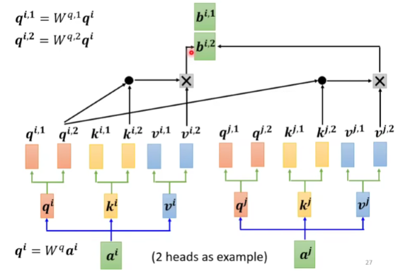
为了防止 decoder 作弊,在计算注意力分数时我们采用 future masking 的策略: \[ \alpha_{i,j,\text{masked}}= \begin{cases} \alpha_{ij} \ \ j\leq i \\ 0 \ \ \ \ \ \text{otherwise} \end{cases} \] Multi-head Self-Attention. 类似 CNN 中的多卷积核与多通道,对同一个输入 \(X\in R^{n\times d}\),多头自注意力进行多次 self-attention,每个头有独立的 \(W_k^{(l)}, W_q^{(l)}, W_v^{(l)}\) 参数 (一个等价的理解是,共用 \(W_k,W_q,W_v\) 但是最后将得到的 \(q,k,v\) 切分成若干个头),并各自独立的得到关注不同特征的 representation。
最后再将每个头得到的结果 \(\text{concat}\) (简单的连接) 起来,再乘上一个转换矩阵 \(W_o\) 得到最终结果。
Layer normalization. 是一个我尝试理解但是失败了的玄学方法。我们知道 stacked self-attention blocks 把 \(x_{1:n}\) 一层一层往上传,LN 通常加在两个 self-attention blocks 之间,normalize each token over all dimensions。
LN 对 token 本身进行 normalization,token 间互不影响,这是 Layer norm 与 Batch norm 的最大区别。若某个 self-attention block 的输出为 \(h\in R^{n,d}\),想象 LN 对行而不是对列进行 normalization,共 \(n\) 次。
Add & Norm. 将 Residual Connections 加入 LN。残差连接的 intuition - identity function 的梯度为 \(1\),缓解了深度神经网络的梯度消失问题;从 identity function 开始学理论上也能够加速找到最优解的过程。
输入 \(h_{1:n}\),Add & Norm
block 执行以下操作:其中 \(f\) 可以是
FFN 甚至 self-attention。 \[
h_{\text{pre-norm}}=f(\text{LN}(h))+h
\]
Transformer
现在 Transformer 的所有关键 components 都已经介绍完毕了,可以开始拼图了!
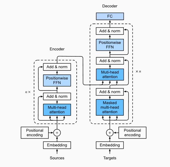
- encoder 是编码模型。encoder-only 的架构常用于生成高质量的 contextual representation,因此不需要对 self-attention 应用 future masking。
- decoder 是自回归的语言模型 (autoregressive language model)。侧重于生成,需要应用 future masking。
- 在 encoder-decoder 架构中,encoder 与 decoder 通过 cross attention 连接。交叉注意力本质上是对自注意力之前的 attention 概念的回归,即 encoder 提供 keys 与 values,decoder 提供 queries。
encoder-decoder transformer 常用于对 bidirectional context 有着较高要求的应用,例如文本总结,机器翻译;但由于需要向 encoder 与 decoder 分配参数,它的深度没法做到 decoder-only transformer 那么深。
时下最流行的 transformer 均是 decoder-only 的,如 GPT (generative pretrained transformer) 系列模型。
Reference
This article is a self-administered course note.
References in the article are from corresponding course materials if not specified.
Course info: Stanford CS224N NLP with Deep Learning (2021~2023)
Lecturer: Prof. Christopher Manning